
Table of Contents
Implementation of Vision Transformer, a simple way to achieve SOTA in vision classification with only a single transformer encoder, in Pytorch. Significance is further explained in Yannic Kilcher's video. There's really not much to code here, but may as well lay it out for everyone so we expedite the attention revolution.
For a Pytorch implementation with pretrained models, please see Ross Wightman's repository here.
The official Jax repository is here.
A tensorflow2 translation also exists here, created by research scientist Junho Kim! 🙏
Flax translation by Enrico Shippole!
Install
$ pip install vit-pytorch
Usage
import torch
from vit_pytorch import ViT

v = ViT(
    image_size = 256,
    patch_size = 32,
    num_classes = 1000,
    dim = 1024,
    depth = 6,
    heads = 16,
    mlp_dim = 2048,
    dropout = 0.1,
    emb_dropout = 0.1
)

img = torch.randn(1, 3, 256, 256)

preds = v(img) # (1, 1000)
Parameters
image_size: int.
Image size. If you have rectangular images, make sure your image size is the maximum of the width and heightpatch_size: int.
Size of patches. image_size must be divisible by patch_size.
The number of patches is: n = (image_size // patch_size) ** 2 and n must be greater than 16.num_classes: int.
Number of classes to classify.dim: int.
Last dimension of output tensor after linear transformation nn.Linear(..., dim).depth: int.
Number of Transformer blocks.heads: int.
Number of heads in Multi-head Attention layer.mlp_dim: int.
Dimension of the MLP (FeedForward) layer.channels: int, default 3.
Number of image's channels.dropout: float between [0, 1], default 0..
Dropout rate.emb_dropout: float between [0, 1], default 0.
Embedding dropout rate.pool: string, either cls token pooling or mean pooling
Simple ViT
An update from some of the same authors of the original paper proposes simplifications to ViT that allows it to train faster and better.
Among these simplifications include 2d sinusoidal positional embedding, global average pooling (no CLS token), no dropout, batch sizes of 1024 rather than 4096, and use of RandAugment and MixUp augmentations. They also show that a simple linear at the end is not significantly worse than the original MLP head
You can use it by importing the SimpleViT as shown below
import torch
from vit_pytorch import SimpleViT

v = SimpleViT(
    image_size = 256,
    patch_size = 32,
    num_classes = 1000,
    dim = 1024,
    depth = 6,
    heads = 16,
    mlp_dim = 2048
)

img = torch.randn(1, 3, 256, 256)

preds = v(img) # (1, 1000)
NaViT
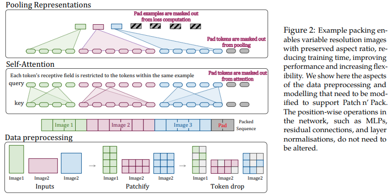
This paper proposes to leverage the flexibility of attention and masking for variable lengthed sequences to train images of multiple resolution, packed into a single batch. They demonstrate much faster training and improved accuracies, with the only cost being extra complexity in the architecture and dataloading. They use factorized 2d positional encodings, token dropping, as well as query-key normalization.
You can use it as follows
import torch
from vit_pytorch.na_vit import NaViT

v = NaViT(
    image_size = 256,
    patch_size = 32,
    num_classes = 1000,
    dim = 1024,
    depth = 6,
    heads = 16,
    mlp_dim = 2048,
    dropout = 0.1,
    emb_dropout = 0.1,
    token_dropout_prob = 0.1  # token dropout of 10% (keep 90% of tokens)
)

# 5 images of different resolutions - List[List[Tensor]]

# for now, you'll have to correctly place images in same batch element as to not exceed maximum allowed sequence length for self-attention w/ masking

images = [
    [torch.randn(3, 256, 256), torch.randn(3, 128, 128)],
    [torch.randn(3, 128, 256), torch.randn(3, 256, 128)],
    [torch.randn(3, 64, 256)]
]

preds = v(images) # (5, 1000) - 5, because 5 images of different resolution above
Or if you would rather that the framework auto group the images into variable lengthed sequences that do not exceed a certain max length
images = [
    torch.randn(3, 256, 256),
    torch.randn(3, 128, 128),
    torch.randn(3, 128, 256),
    torch.randn(3, 256, 128),
    torch.randn(3, 64, 256)
]

preds = v(
    images,
    group_images = True,
    group_max_seq_len = 64
) # (5, 1000)
Finally, if you would like to make use of a flavor of NaViT using nested tensors (which will omit a lot of the masking and padding altogether), make sure you are on version 2.5 and import as follows
import torch
from vit_pytorch.na_vit_nested_tensor import NaViT

v = NaViT(
    image_size = 256,
    patch_size = 32,
    num_classes = 1000,
    dim = 1024,
    depth = 6,
    heads = 16,
    mlp_dim = 2048,
    dropout = 0.,
    emb_dropout = 0.,
    token_dropout_prob = 0.1
)

# 5 images of different resolutions - List[Tensor]

images = [
    torch.randn(3, 256, 256), torch.randn(3, 128, 128),
    torch.randn(3, 128, 256), torch.randn(3, 256, 128),
    torch.randn(3, 64, 256)
]

preds = v(images)

assert preds.shape == (5, 1000)
Distillation
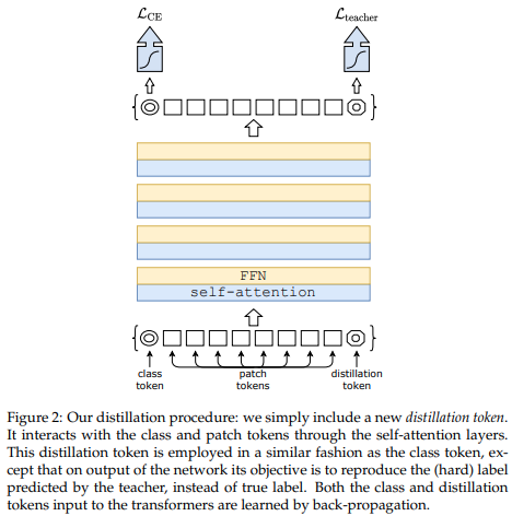
A recent paper has shown that use of a distillation token for distilling knowledge from convolutional nets to vision transformer can yield small and efficient vision transformers. This repository offers the means to do distillation easily.
ex. distilling from Resnet50 (or any teacher) to a vision transformer
import torch
from torchvision.models import resnet50

from vit_pytorch.distill import DistillableViT, DistillWrapper

teacher = resnet50(pretrained = True)

v = DistillableViT(
    image_size = 256,
    patch_size = 32,
    num_classes = 1000,
    dim = 1024,
    depth = 6,
    heads = 8,
    mlp_dim = 2048,
    dropout = 0.1,
    emb_dropout = 0.1
)

distiller = DistillWrapper(
    student = v,
    teacher = teacher,
    temperature = 3,           # temperature of distillation
    alpha = 0.5,               # trade between main loss and distillation loss
    hard = False               # whether to use soft or hard distillation
)

img = torch.randn(2, 3, 256, 256)
labels = torch.randint(0, 1000, (2,))

loss = distiller(img, labels)
loss.backward()

# after lots of training above ...

pred = v(img) # (2, 1000)
The DistillableViT class is identical to ViT except for how the forward pass is handled, so you should be able to load the parameters back to ViT after you have completed distillation training.
You can also use the handy .to_vit method on the DistillableViT instance to get back a ViT instance.
v = v.to_vit()
type(v) # <class 'vit_pytorch.vit_pytorch.ViT'>
Deep ViT
This paper notes that ViT struggles to attend at greater depths (past 12 layers), and suggests mixing the attention of each head post-softmax as a solution, dubbed Re-attention. The results line up with the Talking Heads paper from NLP.
You can use it as follows
import torch
from vit_pytorch.deepvit import DeepViT

v = DeepViT(
    image_size = 256,
    patch_size = 32,
    num_classes = 1000,
    dim = 1024,
    depth = 6,
    heads = 16,
    mlp_dim = 2048,
    dropout = 0.1,
    emb_dropout = 0.1
)

img = torch.randn(1, 3, 256, 256)

preds = v(img) # (1, 1000)
CaiT
This paper also notes difficulty in training vision transformers at greater depths and proposes two solutions. First it proposes to do per-channel multiplication of the output of the residual block. Second, it proposes to have the patches attend to one another, and only allow the CLS token to attend to the patches in the last few layers.
They also add Talking Heads, noting improvements
You can use this scheme as follows
import torch
from vit_pytorch.cait import CaiT

v = CaiT(
    image_size = 256,
    patch_size = 32,
    num_classes = 1000,
    dim = 1024,
    depth = 12,             # depth of transformer for patch to patch attention only
    cls_depth = 2,          # depth of cross attention of CLS tokens to patch
    heads = 16,
    mlp_dim = 2048,
    dropout = 0.1,
    emb_dropout = 0.1,
    layer_dropout = 0.05    # randomly dropout 5% of the layers
)

img = torch.randn(1, 3, 256, 256)

preds = v(img) # (1, 1000)
Token-to-Token ViT
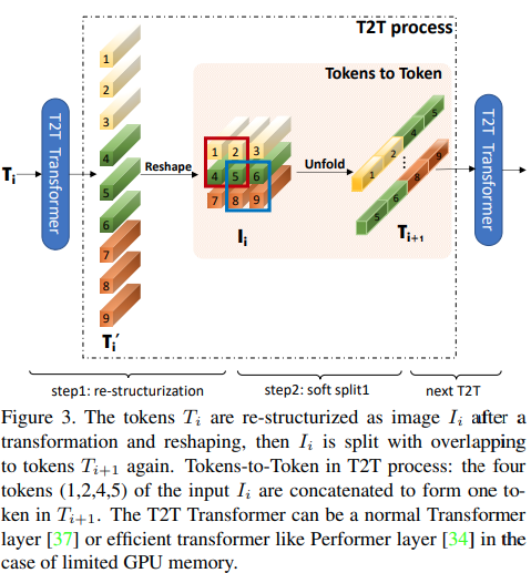
This paper proposes that the first couple layers should downsample the image sequence by unfolding, leading to overlapping image data in each token as shown in the figure above. You can use this variant of the ViT as follows.
import torch
from vit_pytorch.t2t import T2TViT

v = T2TViT(
    dim = 512,
    image_size = 224,
    depth = 5,
    heads = 8,
    mlp_dim = 512,
    num_classes = 1000,
    t2t_layers = ((7, 4), (3, 2), (3, 2)) # tuples of the kernel size and stride of each consecutive layers of the initial token to token module
)

img = torch.randn(1, 3, 224, 224)

preds = v(img) # (1, 1000)
CCT
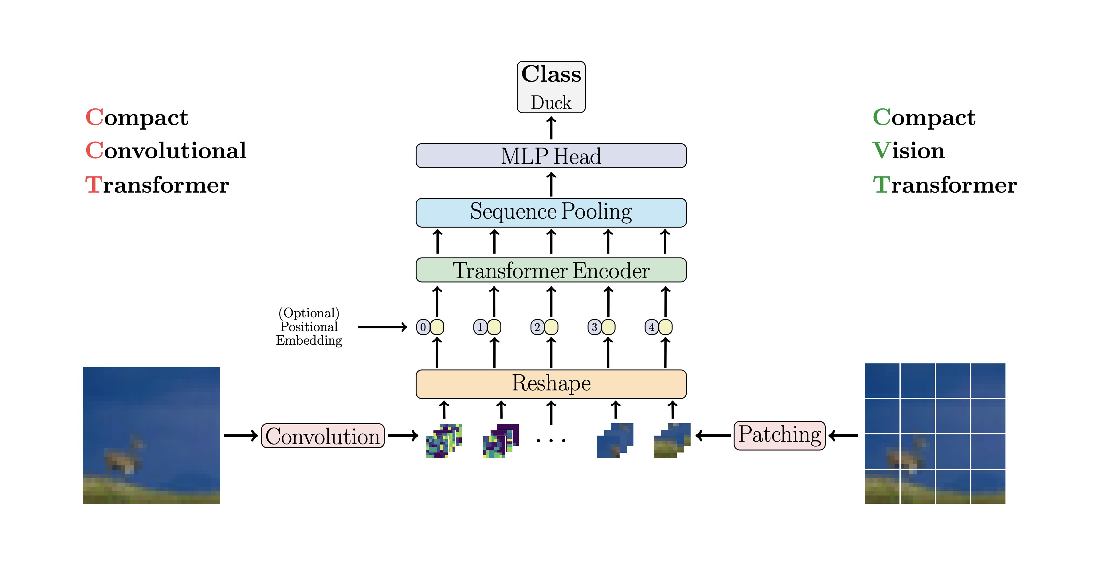
CCT proposes compact transformers
by using convolutions instead of patching and performing sequence pooling. This
allows for CCT to have high accuracy and a low number of parameters.
You can use this with two methods
import torch
from vit_pytorch.cct import CCT

cct = CCT(
    img_size = (224, 448),
    embedding_dim = 384,
    n_conv_layers = 2,
    kernel_size = 7,
    stride = 2,
    padding = 3,
    pooling_kernel_size = 3,
    pooling_stride = 2,
    pooling_padding = 1,
    num_layers = 14,
    num_heads = 6,
    mlp_ratio = 3.,
    num_classes = 1000,
    positional_embedding = 'learnable', # ['sine', 'learnable', 'none']
)

img = torch.randn(1, 3, 224, 448)
pred = cct(img) # (1, 1000)
Alternatively you can use one of several pre-defined models [2,4,6,7,8,14,16]
which pre-define the number of layers, number of attention heads, the mlp ratio,
and the embedding dimension.
import torch
from vit_pytorch.cct import cct_14

cct = cct_14(
    img_size = 224,
    n_conv_layers = 1,
    kernel_size = 7,
    stride = 2,
    padding = 3,
    pooling_kernel_size = 3,
    pooling_stride = 2,
    pooling_padding = 1,
    num_classes = 1000,
    positional_embedding = 'learnable', # ['sine', 'learnable', 'none']
)
Official
Repository includes links to pretrained model checkpoints.
Cross ViT

This paper proposes to have two vision transformers processing the image at different scales, cross attending to one every so often. They show improvements on top of the base vision transformer.
import torch
from vit_pytorch.cross_vit import CrossViT

v = CrossViT(
    image_size = 256,
    num_classes = 1000,
    depth = 4,               # number of multi-scale encoding blocks
    sm_dim = 192,            # high res dimension
    sm_patch_size = 16,      # high res patch size (should be smaller than lg_patch_size)
    sm_enc_depth = 2,        # high res depth
    sm_enc_heads = 8,        # high res heads
    sm_enc_mlp_dim = 2048,   # high res feedforward dimension
    lg_dim = 384,            # low res dimension
    lg_patch_size = 64,      # low res patch size
    lg_enc_depth = 3,        # low res depth
    lg_enc_heads = 8,        # low res heads
    lg_enc_mlp_dim = 2048,   # low res feedforward dimensions
    cross_attn_depth = 2,    # cross attention rounds
    cross_attn_heads = 8,    # cross attention heads
    dropout = 0.1,
    emb_dropout = 0.1
)

img = torch.randn(1, 3, 256, 256)

pred = v(img) # (1, 1000)
PiT
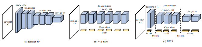
This paper proposes to downsample the tokens through a pooling procedure using depth-wise convolutions.
import torch
from vit_pytorch.pit import PiT

v = PiT(
    image_size = 224,
    patch_size = 14,
    dim = 256,
    num_classes = 1000,
    depth = (3, 3, 3),     # list of depths, indicating the number of rounds of each stage before a downsample
    heads = 16,
    mlp_dim = 2048,
    dropout = 0.1,
    emb_dropout = 0.1
)

# forward pass now returns predictions and the attention maps

img = torch.randn(1, 3, 224, 224)

preds = v(img) # (1, 1000)
LeViT
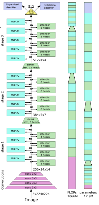
This paper proposes a number of changes, including (1) convolutional embedding instead of patch-wise projection (2) downsampling in stages (3) extra non-linearity in attention (4) 2d relative positional biases instead of initial absolute positional bias (5) batchnorm in place of layernorm.
Official repository
import torch
from vit_pytorch.levit import LeViT

levit = LeViT(
    image_size = 224,
    num_classes = 1000,
    stages = 3,             # number of stages
    dim = (256, 384, 512),  # dimensions at each stage
    depth = 4,              # transformer of depth 4 at each stage
    heads = (4, 6, 8),      # heads at each stage
    mlp_mult = 2,
    dropout = 0.1
)

img = torch.randn(1, 3, 224, 224)

levit(img) # (1, 1000)
CvT
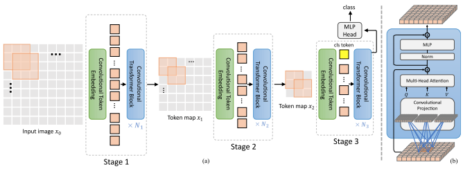
This paper proposes mixing convolutions and attention. Specifically, convolutions are used to embed and downsample the image / feature map in three stages. Depthwise-convoltion is also used to project the queries, keys, and values for attention.
import torch
from vit_pytorch.cvt import CvT

v = CvT(
    num_classes = 1000,
    s1_emb_dim = 64,        # stage 1 - dimension
    s1_emb_kernel = 7,      # stage 1 - conv kernel
    s1_emb_stride = 4,      # stage 1 - conv stride
    s1_proj_kernel = 3,     # stage 1 - attention ds-conv kernel size
    s1_kv_proj_stride = 2,  # stage 1 - attention key / value projection stride
    s1_heads = 1,           # stage 1 - heads
    s1_depth = 1,           # stage 1 - depth
    s1_mlp_mult = 4,        # stage 1 - feedforward expansion factor
    s2_emb_dim = 192,       # stage 2 - (same as above)
    s2_emb_kernel = 3,
    s2_emb_stride = 2,
    s2_proj_kernel = 3,
    s2_kv_proj_stride = 2,
    s2_heads = 3,
    s2_depth = 2,
    s2_mlp_mult = 4,
    s3_emb_dim = 384,       # stage 3 - (same as above)
    s3_emb_kernel = 3,
    s3_emb_stride = 2,
    s3_proj_kernel = 3,
    s3_kv_proj_stride = 2,
    s3_heads = 4,
    s3_depth = 10,
    s3_mlp_mult = 4,
    dropout = 0.
)

img = torch.randn(1, 3, 224, 224)

pred = v(img) # (1, 1000)
Twins SVT
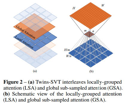
This paper proposes mixing local and global attention, along with position encoding generator (proposed in CPVT) and global average pooling, to achieve the same results as Swin, without the extra complexity of shifted windows, CLS tokens, nor positional embeddings.
import torch
from vit_pytorch.twins_svt import TwinsSVT

model = TwinsSVT(
    num_classes = 1000,       # number of output classes
    s1_emb_dim = 64,          # stage 1 - patch embedding projected dimension
    s1_patch_size = 4,        # stage 1 - patch size for patch embedding
    s1_local_patch_size = 7,  # stage 1 - patch size for local attention
    s1_global_k = 7,          # stage 1 - global attention key / value reduction factor, defaults to 7 as specified in paper
    s1_depth = 1,             # stage 1 - number of transformer blocks (local attn -> ff -> global attn -> ff)
    s2_emb_dim = 128,         # stage 2 (same as above)
    s2_patch_size = 2,
    s2_local_patch_size = 7,
    s2_global_k = 7,
    s2_depth = 1,
    s3_emb_dim = 256,         # stage 3 (same as above)
    s3_patch_size = 2,
    s3_local_patch_size = 7,
    s3_global_k = 7,
    s3_depth = 5,
    s4_emb_dim = 512,         # stage 4 (same as above)
    s4_patch_size = 2,
    s4_local_patch_size = 7,
    s4_global_k = 7,
    s4_depth = 4,
    peg_kernel_size = 3,      # positional encoding generator kernel size
    dropout = 0.              # dropout
)

img = torch.randn(1, 3, 224, 224)

pred = model(img) # (1, 1000)
RegionViT
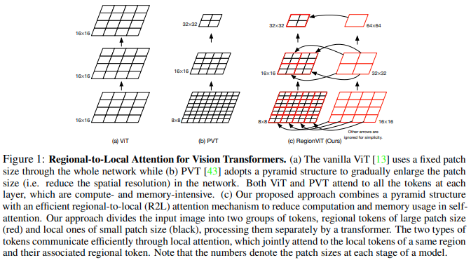
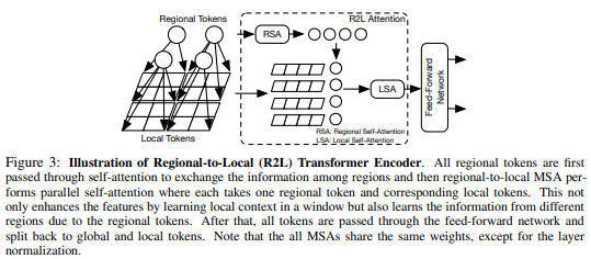
This paper proposes to divide up the feature map into local regions, whereby the local tokens attend to each other. Each local region has its own regional token which then attends to all its local tokens, as well as other regional tokens.
You can use it as follows
import torch
from vit_pytorch.regionvit import RegionViT

model = RegionViT(
    dim = (64, 128, 256, 512),      # tuple of size 4, indicating dimension at each stage
    depth = (2, 2, 8, 2),           # depth of the region to local transformer at each stage
    window_size = 7,                # window size, which should be either 7 or 14
    num_classes = 1000,             # number of output classes
    tokenize_local_3_conv = False,  # whether to

 A PyTorch implementation of the Vision Transformer (ViT), an image classification model that reaches SOTA results using just a single transformer encoder instead of convolutions.